The ELS optical fleximeter allows recording the deformation that a sample suspended between two supports undergoes when the viscosity is sufficiently reduced to allow flow caused by its own weight.

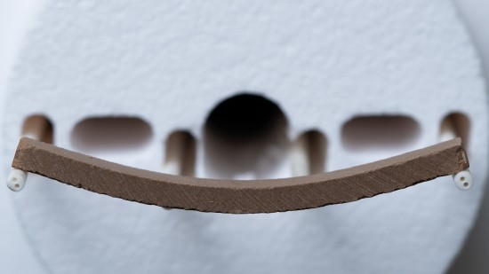
The image shows a porcelain tile sample, brought to a temperature such as to trigger the flow of the vitreous phases contained in the ceramic matrix.

In glasses, and materials containing similar amorphous phases, viscosity undergoes a rapid decrease starting from the glass transition, after which the drop becomes exponential.
The viscosity decrease follows the Vogel-Fulcher-Tamman (VFT) equation already discussed in this case study (), where it was explained how it is possible to deduce the temperatures corresponding to some precise viscosity values by combining different techniques (optical dilatometer and heating microscope).

$$ \log\eta = A + \frac{B}{T - T_0} $$

In this study it will be demonstrated how it is possible to calculate viscosity from the fleximetry curve, directly applying well-known equations from literature.

In Treatise on Mathematical Theory of Elasticity (1944) the author (Love) starts from first principles to calculate the deflection caused by the elasticity of the material in the case of a bar deformed by its own weight (Article 247 b).
McDowall & Vose (1951) and subsequently Adcock, Drummond, McDowall (1959) adapt Love’s treatment to viscous flow, deriving the equation that relates viscosity $\eta$ and deformation rate at the center of the sample $\dot{s}$ in the case of a rod of diameter d, suspended between two supports distant L and having density $\rho$:

$$ \eta = \frac{5 \rho g L^4}{72 d^2 \dot{s}} $$

Where g is the gravitational acceleration constant.
Similar equations are also available for other geometries, including that relating to the rectangular bar, where instead of the diameter the thickness of the bar is considered and the entire formula is multiplied by $\frac{3}{4}$ (in the denominator there is 96 instead of 72).
The deformation rate can be obtained by deriving the fleximetry curve with respect to time, while all other variables of the equation can be easily determined at room temperature and, as a first approximation, approximated as constants.
Having a dilatometric curve for the same temperature interval, it is possible to correct the thickness of the rod by applying the same percentage expansion point by point.
As the sample deforms due to gravity, it also tends to elongate on a parabolic arc P at the expense of its thickness, according to the parabolic arc equation:

$$ P = \frac{1}{2} \sqrt{L^2 + 16s^2} \frac{L^2}{8s} \ln \left( \frac{4s + \sqrt{L^2 + 16s^2}}{L} \right) $$

Each increase in parabolic length P=L+dL must be compensated by a decrease in radius by a factor a in the new corrected radius r$_{1}$=ar to preserve the volume V=V$_{1}$:

$$ V = L\pi r^2; \quad V_1 = (L+dL) \pi (ar)^2; \quad V_1=V $$

$$ P \pi (a r)^2 = L\pi r^2 $$

$$ a = \sqrt{\frac{L}{P}} $$

The same factor also applies to the diameter correction, and also in the case of the rectangular section having thickness d and depth b:

$$ V = Ldb; \quad V_1 = (L+dL)a^2 db $$

$$ Pa^2 db = Ldb $$

$$ a = \sqrt{\frac{L}{P}} $$

Knowing the thermal expansion it is also possible to correct the density, which decreases as the volume of the material increases. If the sample undergoes weight variations, due to decompositions, oxidations and other chemical reactions, it is possible to record a thermogravimetric curve in percentage and multiply it by the density, correcting it further.

Experimental procedure

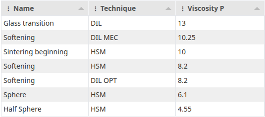
McDowall’s equation, including the corrections discussed here, was verified on an industrial sample of DURAN glass (Schott), in the form of a solid rod with a diameter of 5mm. For this material the supplier publishes the following characteristic temperatures:

• Annealing, 10$^{13}$dPa·s (Poise), 560°C
• Softening, 10$^{7.6}$dPa·s, 825°C
• Working, 10$^{4}$dPa·s, 1260°C

Thus allowing to solve the VFT equation and evaluate the viscosity within the entire temperature range 500-1300°C with confidence.
The rod was subjected to the following heating cycle:

• 80°C/min up to 500°C
• 20°C/min up to 550°C
• 5°C/min up to 750°C

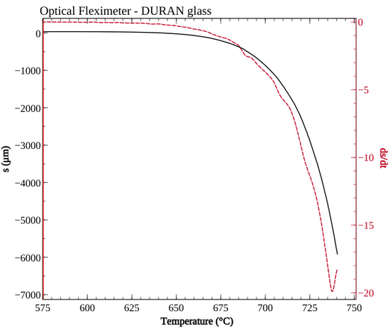
The deformation begins at 590°C and is automatically interrupted at 740°C due to exceeding the instrument’s field of view (6mm).
The following graph shows the bending curve and its derivative with respect to time.

The expansion curve is measured with the differential optical dilatometer. This technique guarantees maximum precision and reproducibility thanks to real-time calibration, enabled by the simultaneous measurement of a reference standard.

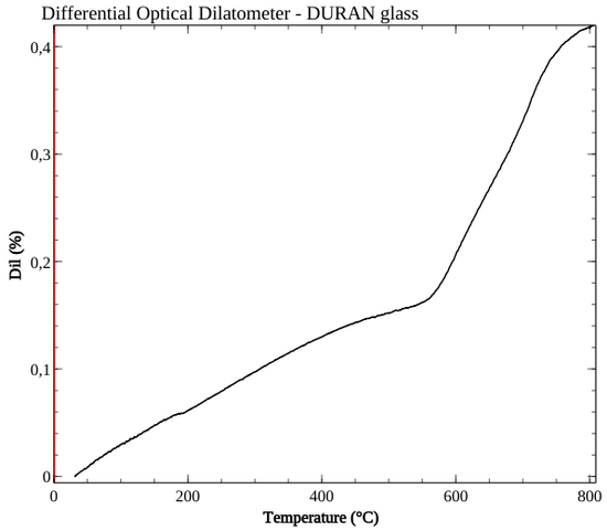
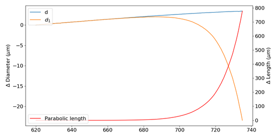
The parabolic length reaches a deviation of almost 1 mm at the maximum bending of 6mm. The consequent correction of the initial diameter proves to be of little relevance: the maximum discrepancy between the diameter increased due to the expansion effect (+3μm) and that contracted due to the parabolic elongation at constant volume (-25μm) is only 28μm, as highlighted in the following graph.

Viscosity calculation

Once the effective thickness and density are obtained by combining thermal expansion and bending, one can proceed to derive the bending curve with respect to time and solve the McDowall & Vose formula starting from the first detectable deformation.
Since the deformation rate is in the denominator, the resulting viscosity curve is numerically unstable at low temperatures due to the imperceptible deformation and even more uncertain velocity. It is necessary to wait for 620°C for the velocity to be sufficiently sustained to stabilize the calculated viscosity.
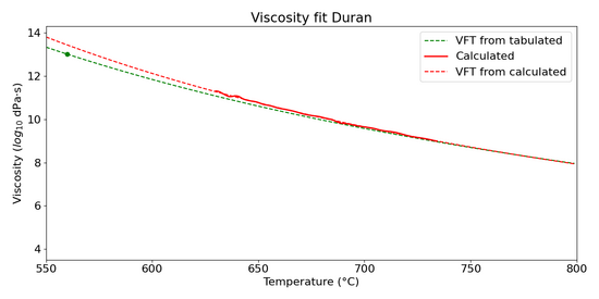
As can be appreciated from the logarithmic representation, the curve is exponential — what would be expected from a viscosity that responds to the VFT equation.

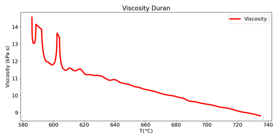
It can also be appreciated that the instrumental limits reduce the applicability of this technique to the viscosity range between 10$^{12}$ and 10$^{9}$ dPa·s, i.e. between the annealing and softening of glasses.
At higher viscosities the deformation is too slow to be appreciable (at this heating rate, i.e. 5°C/min) while at values below the lower margin the deformation is so rapid as to exit the instrumental margins in a few seconds.
The range is technologically relevant for many applications, from glass processing to firing of tiles, tableware and ceramic sanitary ware, as well as for studying the creep of metals at high temperature, in the new ELS-MDF instrument models with controlled atmosphere.

The viscosity curve derived from the optical fleximeter was then compared with the VFT interpolation from the values tabulated by the supplier (green curve), finding excellent agreement in the temperature range considered.
The following table shows the comparison between the VFT parameters from tabulated and from measured viscosity points:

Parameter	Tabulated	Measured
Pre-exponential, A	-2.154	-2.33
Exponent, B	7255.8	7054.5
Activation, T$_{0}$	81.29	111.37

The following table instead shows a comparison between the viscosity values (log$_{10}$ dPa·s) interpolated from the tabulated data using the VFT and those measured directly.

Temperature (°C)	Tabulated	Measured
550	13.32	13.74
560	13.00	13.38
570	12.69	13.04
580	12.39	12.71
590	12.11	12.40
600	11.83	12.10
610	11.57	11.81
620	11.31	11.53
630	11.07	11.26
640	10.83	11.01
650	10.60	10.76
660	10.38	10.52
670	10.17	10.29
680	9.96	10.07
690	9.76	9.85
700	9.57	9.64
710	9.38	9.44
720	9.20	9.25
730	9.03	9.06
740	8.86	8.88
750	8.69	8.71
760	8.53	8.54
770	8.38	8.37
780	8.23	8.21
790	8.08	8.06

Conclusions

The combination of optical fleximeter and differential optical dilatometer can be successfully employed to calculate the viscosity of materials subjected to heating in the range between 10$^{12}$ and 10$^{9}$ dPa·s, important for many industrial applications.

The technique was verified on DURAN industrial glass from Schott, showing good agreement, and further tests will be conducted on a certified standard material as soon as available.

Having a viscosity curve derived from a direct measurement, through fitting of the McDowall & Vose mechanical model, allows accurate comparisons between inhomogeneous materials and under different experimental conditions.

The measurement does not depend on characteristic points whose viscosity must already be known in literature, as occurs to be able to apply the calculation according to VFT. The new technique therefore allows studying even non-vitreous materials or those that do not respond perfectly to that model, for example in the case where solid-state reactions or dissolutions of crystalline phases intervene that modify the viscosity independently of temperature. Thus accurate viscosity measurement becomes possible even for traditional ceramics composed of multiple crystalline phases evolving during the thermal cycle.